Dasymetric Spatial Interpolation in BigQuery
Mapping census population to H3 hexagons
In my current job at Unacast, we transform large amounts of locational data and often times aggregate metrics based on administrative areas. But these areas vary in size and distribution of population, which makes them less suitable for normalizing mobility metrics or comparing areas with each other. Dasymetric spatial interpolation can mitigate this issue to a large degree, a and a spatial index gaining popularity is Uber's H3 hexagons.
During the Spatial Data Science Conference 2020 organized by Carto, Daniel Arribas-Bel and John Levi displayed a quick example of a dasymetric map using census population and H3 hexagons with Python, alongside introducing their upcoming book "Geographic Data Science with PySAL and the PyData Stack". At Unacast we work mostly in BigQuery. I therefore want to demonstrate how to achieve spatial interpolation -similar to some of the functionalities provided in Python- using BigQueries powerful geospatial functions.
I will show 3 different approaches:
- A simple spatial interpolation based on area overlap
- A dasymetric interpolation using Open Street Map data
- Dasymetric interpolation using parcel information
I will demonstrate the methodology on one example county in the U.S. (Orange County, Florida). The county consists of several census block groups (CBGs) for which we get population data and polygons of the boundaries through Google's public datasets. Plotting the census block groups as a choropleth using the census population highlights the aforementioned weaknesses of administrative spatial units.

The CBGs in the center are mostly small and often don't feature high absolute population numbers. In contrast, the rural areas have some huge CBGs with high absolute population. It feels counterintuitive to see low population in the city center and high population further out, but it is simple driven by the difference in size of these CBGs. This highlights the appeal of equi-sized spatial units like H3 instantly, we just need to find a way to distribute the population to the hexagons.
Let’s get started with the most simple approach and calculate the interpolated population for each hexagon based on the area overlap with each census block group first. I will use zoom level 7 throughout this post, but the methodology works independently of the zoom level (the title picture was created with zoom level 9). All visualizations are done in kepler.gl.
Going forward, I will make use of the JS library which is incredibly useful when dealing with H3. First, we “fill” the county polygon with hexagons of the specified zoom level 7, and create an array with the corresponding H3 ids using ST_H3_POLYFILLFROMGEOG directly in BigQuery. From here, ST_H3_BOUNDARY returns the polygons for each H3 id:
WITH
  county_polyfill AS(
    SELECT
        jslibs.h3.ST_H3_POLYFILLFROMGEOG(county_geom ,7) as geo
    FROM `bigquery-public-data.geo_us_boundaries.counties`
        WHERE geo_id = '12095'
  ),
  h3_hexagons as (
    SELECT
        h3,
        jslibs.h3.ST_H3_BOUNDARY(h3) as h3geo
    FROM county_polyfill, UNNEST(geo) as h3
  ),
Next, we calculate the overlap of each hexagon with the census block groups it intersects.
geom_overlap AS(
  SELECT
      h3,
      h3geo,
      geo_id,
      total_pop,
      ST_AREA(ST_INTERSECTION(h3geo, blockgroup_geom)) as intersection_h3,
      ST_AREA(blockgroup_geom) as cbg_area
  FROM h3_hexagons
    JOIN `bigquery-public-data.geo_census_blockgroups.us_blockgroups_national` cbg_geo
      ON ST_INTERSECTS(h3geo, blockgroup_geom)
    JOIN `bigquery-public-data.census_bureau_acs.blockgroup_2018_5yr` cbg_pop
      USING(geo_id)
  )
In the last step, the population for each hexagon is summed up, weighted by the overlap as a share of the total area of each census block group.
SELECT
    h3,
    ANY_VALUE(h3geo) as hex_geo,
    SUM(SAFE_DIVIDE(intersection_h3,cbg_area) * total_pop) as h3_pop
FROM geom_overlap
  GROUP BY h3
When plotting the interpolated population we now get the intuitive result that population is concentrated in the city center and density decreases further away from the center.
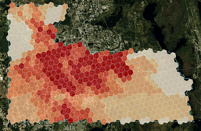
While this solves some of the issues described earlier, the methodology is rather crude in the sense that it assumes the population of each CBG to be equally distributed over space within each CBG. My objective is to get a more accurate distribution of the population even within each CBG.
One way to improve the interpolation is to use supplementary data like satellite images to reduce each CBG to its habitable area. I want to propose two alternatives to satellite images that are publicly available and achieve the same goal, potentially even with a better distinction between building types (commercial/industrial vs. residential).
The first approach uses Open Street Map data (OSM) which is available as a Google public dataset in BigQuery. Extracting the footprint of residential buildings provides a good approximation of the spatial clustering of census population. I will skip the explanation of how to filter for residential buildings in the OSM data as it is by far no exact science and assume a table with the extracted building polygons going forward.
First, the population for each residential housing polygon is calculated based on the overlap of the total residential housing area of each CBG, and the CBG population.
WITH buildings_overlap AS (
  SELECT
      osm.osm_way_id,
      osm.geometry,
      cbg_geo.geo_id,
      cbg_geo.blockgroup_geom,
      ST_AREA(ST_INTERSECTION(blockgroup_geom,osm.geometry)) as intersection_area,
  FROM `my-project.mydataset.buildings_osm` osm
    JOIN `bigquery-public-data.geo_census_blockgroups.us_blockgroups_national` cbg_geo
      ON ST_INTERSECTS(blockgroup_geom, geometry)
  WHERE CONCAT(state_fips_code, county_fips_code) = '12095'
),
--total area of all residential polygons for each CBG
building_area_per_cbg AS (
  SELECT
      geo_id,
      SUM(intersection_area) as building_area_total
  FROM buildings_overlap
  GROUP BY geo_id
),
--population for each overlapping area
share_population_building AS (
  SELECT
    osm_way_id,
    geometry,
    geo_id,
    SAFE_DIVIDE(intersection_area, building_area_total) * total_pop as building_pop_overlap
  FROM buildings_overlap
    JOIN building_area_per_cbg
        USING(geo_id)
    JOIN `bigquery-public-data.census_bureau_acs.blockgroup_2018_5yr`
      USING(geo_id)
),
population_per_building as (
  SELECT
      osm_way_id,
      ANY_VALUE(geometry) as building_geo,
      SUM(building_pop_overlap) as building_pop_total
  FROM share_population_building
  GROUP BY osm_way_id
),
With a metric representing the population assigned to each building polygon, it is now possible to calculate the overlap of each H3 hexagon with each residential building similar to the first approach and aggregate the population up to the hexagon level.
county_polyfill as (
    SELECT
        jslibs.h3.ST_H3_POLYFILLFROMGEOG(county_geom ,7) as geo
    FROM `bigquery-public-data.geo_us_boundaries.counties`
        WHERE geo_id = '12095'
  ),
  h3_hexagons as (
    SELECT
        h3,
        jslibs.h3.ST_H3_BOUNDARY(h3) as h3geo
    FROM county_polyfill, UNNEST(geo) as h3
  ),
--overlap of each H3 hexagon with each building
geom_overlap as (
SELECT
    h3,
    h3geo,
    osm_way_id,
    ST_AREA(ST_INTERSECTION(building_geo, h3geo)) as intersection_h3,
    ST_AREA(building_geo) as building_area,
    building_pop_total
FROM h3_hexagons
  JOIN population_per_building
    ON ST_INTERSECTS(building_geo, h3geo)
)
SELECT
    h3,
    ANY_VALUE(h3geo) as hex_geo,
    SUM(SAFE_DIVIDE(intersection_h3,building_area) * building_pop_total) as h3_pop
FROM geom_overlap
GROUP BY h3
Finally, the results are visualized (Hexagons with a population of zero are left out).
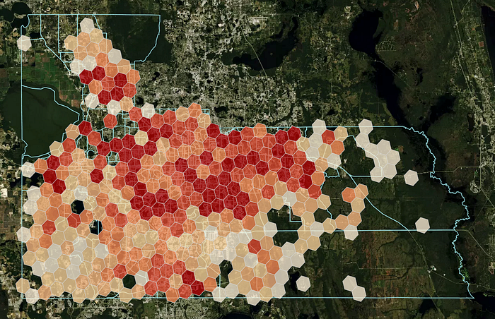
You can see in the visualisation that some quite intuitive results for census block groups in the east and south east corner of the county appear. When inspecting the satellite picture of the base map, what seems to be open space does not get population assigned and any remaining population is clustered around the road network. But a weakness of OSM data also becomes apparent. OSM polygon coverage is not 100% reliable as is visible in the north west of the county. Spot checking directly in the OSM web UI shows that houses in these neighborhoods are simply not present as polygons in the OSM data.
This leads to the last approach. Instead of residential housing polygons, we use another source of information to determine where residents are located which is parcels and their land use code. Parcel data is openly available, yet usually only for an administrative area at a time and it requires some additional time to find it, transform it, load it into BigQuery etc.. Luckily at Unacast I have access to nationwide parcel information.
The methodology part is just a slight variation of the approach using OSM: instead of building polygons, parcel polygons with a residential- or related land use code are used in the calculation. Otherwise the methodology follows the same steps as before. It's best to fast-forward and plot the result at this point.
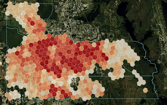
The parcel approach filters out uninhabited areas like agricultural land or the airport (in the bottom center). At the same time we enjoy better coverage than OSM in the north-east part of the county. The comparison across all approaches supports the parcel solution as the winner.


Now that we have these methodologies covered it seems like a good idea to quickly summarize some of the implicit assumptions of each approach:
- Simple overlap - assumption: population is equally distributed over space within each CBG
- OSM building polygon approach- assumption: population increases linearly with building area within CBG
- Parcel polygon approach- assumption: population increases linearly with parcel area within CBG
The assumption of a linear increase in population with building or parcel area size sounds somewhat strong at first: a skyscraper and a large single-family villa might have a similar size footprint yet very different resident counts. But this assumption is spatially bounded to hold only within a CBG. You rarely see the skyscraper and the villa close to each other and the assumption that housing units are of somewhat similar type within each CBG is holds to a large degree.
In the future I might explore some applications of this spatial interpolation and if something interesting arises I might follow up with another article, but I would be happy to hear from other people if they incorporated an approach like this into any of their projects.
Sources:
Dasymetric maps: https://en.wikipedia.org/wiki/Dasymetric_map
H3: https://eng.uber.com/h3/
JS library: https://github.com/CartoDB/bigquery-jslibs
Carto: https://spatial-data-science-conference.com/
Open Street Map: https://www.openstreetmap.org/
BigQuery Geography functions: https://cloud.google.com/bigquery/docs/reference/standard-sql/geography_functions
Kepler: https://kepler.gl/
BigQuery public datasets: https://cloud.google.com/bigquery/public-data
Geospatial data science: https://geographicdata.science/book/intro.html